Filling Atomic Orbitals with Electrons

The energy of an electron depends on the type of orbital that it occupies. Most of the organic compounds that we will encounter will be composed of first- and second-row elements (H, C, N, and O). These elements utilize the 1s  orbital, the 2s  orbital, and the three 2p  orbitals. Our discussions will therefore focus primarily on these orbitals. Electrons are lowest in energy when they occupy a 1s  orbital, because the 1s  orbital is closest to the nucleus and it has no nodes (the more nodes that an orbital has, the greater its energy). The 2s  orbital has one node and is farther away form the nucleus; it is therefore higher in energy than the 1s  orbital. After the 2s  orbital, there are three 2p  orbitals that are all equivalent in energy to one another. Orbitals with the same energy level are called degenerate orbitals .

 

As we move across the periodic table, starting with hydrogen, each element has one more electron than the element before it. The order in which the orbitals are filled by electrons is determined by just three simple principles:

1. The  Aufbau principle. The lowest-energy orbital is filled first.

2. The  Pauli exclusion principle. Each orbital can accommodate a maximum of two electrons that have opposite spin. To understand what “spin” means, we can imagine an electron spinning in space (although this is an oversimplified explanation of the term “spin”). For reasons that are beyond the scope of this course, electrons only have two possible spin states (designated by  or  ). In order for the orbital to accommodate two electrons, the electrons must have opposite spin states.

3. Hund’s Rule. When dealing with degenerate orbitals, such as p orbitals, one electron is placed in each degenerate orbital first, before electrons are paired up. The application of the first two principles can be seen in the electron configurations shown in  (H, He, Li, and Be). The application of the third principle can be seen in the electron configurations for the remaining second-row elements.

 

 

Atomic Orbitals

Quantum Mechanics

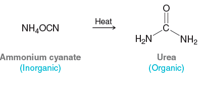
     By the 1920s, vitalism had been discarded. Chemists were aware of constitutional isomerism and had developed the structural theory of matter. The electron had been discovered and identified as the source of bonding, and Lewis structures were used to keep track of shared and unshared electrons. But the understanding of electrons was about to change dramatically.

In 1924, French physicist Louis de Broglie suggested that electrons, heretofore considered as particles, also exhibited wavelike properties. Based on this assertion, a new theory of matter was born. In 1926, Erwin Schrödinger, Werner Heisenberg, and Paul Dirac independently proposed a mathematical description of the electron that incorporated its wavelike properties. This new theory, called wave mechanics,  or quantum mechanics , radically changed the way we viewed the nature of matter and laid the foundation for our current understanding of electrons and bonds.

Quantum mechanics is deeply rooted in mathematics and represents an entire  subject by itself. The mathematics involved is beyond the scope of our course, and we will not discuss it here. However, in order to understand the nature of electrons, it is critical to understand a few simple highlights from quantum mechanics:

 

— An equation is constructed to describe the total energy of a hydrogen atom (i.e. proton plus one electron). This equation, called the wave equation, takes into account the wavelike behavior of an electron that is in the electric field of a proton.

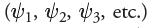
—  The wave equation is then solved to give a series of solutions called wave function . The Greek symbol psi  is used to denote each wave function . Each of these wavefunctions corresponds to an allowed energy level for the electron. This result is incredibly important because it suggests that an electron, when contained in an atom, can only exist at discrete energy levels . In other words, the energy of the electron is quantized.

—  Each wave function is a function of spatial location. It provides information that allows us to assign a numerical value for each location in three-dimensional space relative to the nucleus. The square of that value ( for any particular location) has a special meaning. It indicates the probability of finding the electron in that location. Therefore, a three-dimensional plot of will generate an image of an atomic orbital.

 

Electron Density and Atomic Orbitals

     An orbital  is a region of space that can be occupied by an electron. But care must be taken when trying to visualize this. There is a statement from the previous section that must be clarified because it is potentially misleading: “represents the probability of finding an electron in a particular location .” This statement seems to treat an electron as if it were a particle flying around within a specific region of space. But remember that an electron is not purely a particle—it has wavelike properties as well. Therefore, we must construct a mental image that captures both of these properties. That is not easy to do, but the following analogy might help. We will treat an occupied orbital as if it is a cloud—similar to a cloud in the sky. No analogy is perfect, and there are certainly features of clouds that are very different from orbitals. However, focusing on some of these differences between electron clouds (occupied orbitals) and real clouds makes it possible to construct a better mental model of an electron in an orbital:

— Clouds in the sky can come in any shape or size. However, electron clouds only come in a small number of shapes and sizes (as defined by the orbitals).

— A cloud in the sky is comprised of billions of individual water molecules. An electron cloud is not comprised of billions of particles. We must think of an electron cloud as a single entity, even though it can be thicker in some places and thinner in other places. This concept is critical and will be used extensively throughout the course in explaining reactions.

— A cloud in the sky has edges, and it is possible to define a region of space that contains 100% of the cloud. In contrast, an electron cloud does not have defined edges. We frequently use the term electron density, which is associated with the probability of finding an electron in a particular region of space. The “shape” of an orbital refers to a region of space that contains 90-95% of the electron density.  Beyond this region, the remaining 5-10% of the electron density tapers off but never ends. In fact, if we want to consider the region of space that contains 100% of the electron density,  we must consider the entire universe.

In summary, we must think of an orbital as a region of space that can be occupied by electron density. An occupied orbital must be treated as a cloud of electron density . This region of space is called an atomic orbital  (AO), because it is a region of space defined with respect to the nucleus of a single atom. Examples of atomic orbitals are the s , p , d , and f  orbitals that were discussed in your general chemistry textbook.

Phases of Atomic Orbitals

     Our discussion of electrons and orbitals has been based on the premise that electrons have wavelike properties. As a result, it will be necessary to explore some of the characteristics of simple waves in order to understand some of the characteristics of orbitals.

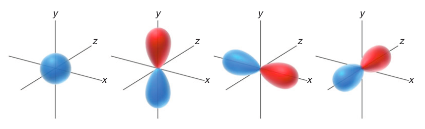
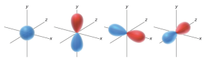
Consider a wave that moves across the surface of a lake. The wave function  mathematically describes the wave, and the value of the wave function is dependent on location. Locations above the average level of the lake have a positive value for  (indicated in red), and locations below the average level of the lake have a negative value for (indicated in blue). Locations where the value of  is zero are called nodes.

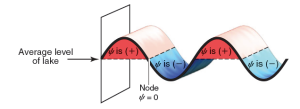
Similarly, orbitals can have regions where the value of  is positive, negative, or zero. For example, consider a p  orbital. Notice that the p  orbital has two lobes: the top lobe is a region of space where the values of  are positive, while the bottom lobe is a region where the values of are negative. Between the two lobes is a location where = 0. This location represents a node.

Be careful not to confuse the sign of  ( + or – ) with electrical charge. A positive value for  does not imply a positive charge. The value of   (+or -) is a mathematical convention that refers to the phase  of the wave (just like in the lake). Although  can have positive or negative values, nevertheless   (which describes the electron density as a function of location) will always be a positive number. At a node, where = 0, the electron density  will also be zero. This means that there is no electron density located at a node. From this point forward, we will draw the lobes of an orbital with colors (red and blue) to indicate the phase of   for each region of space.

 

Electrostatic Potential Maps

Partial charges can be visualized with three-dimensional, rainbow like images called electrostatic potential maps. As an example, consider the electrostatic potential map of chloromethane.

In the image, a color scale is used to represent areas of  and . As indicated, red represents a region that is , while blue represents a region that is . In reality, electrostatic potential maps are rarely used by practicing organic chemists when they communicate with each other; however, these illustrations can often be helpful to students who are learning organic chemistry. Electrostatic potential maps are generated by performing a series of calculations. Specifically, an imaginary point positive charge is positioned at various locations, and for each location, we calculate the potential energy associated with the attraction between the point positive charge and the surrounding electrons. A large attraction indicates a position of , while a small attraction indicates a position of . The results are then illustrated using colors, as shown.

A comparison of any two electrostatic potential maps is only valid if both maps were prepared using the same color scale. Throughout this book, care has been taken to use the same color scale whenever two maps are directly compared to each other. However, it will not be useful to compare two maps from different pages of this book (or any other book), as the exact color scales are likely to be different.

Induction and Polar Covalent Bonds

Chemists classify bonds into three categories: (1) covalent, (2) polar covalent, and (3) ionic. These categories emerge from the electronegativity values of the atoms sharing a bond. Electronegativity  is a measure of the ability of an atom to attract electrons. Table 1.1 gives the electronegativity values for elements commonly encountered in organic chemistry.

When two atoms form a bond, there is one critical question that allows us to classify the bond: What is the difference in the electronegativity values of the two atoms? Below are some rough guidelines:

If the difference in electronegativity is less than 0.5 , the electrons are considered to be equally shared between the two atoms, resulting in a covalent bond. Examples include C–C and C–H:

The C–C bond is clearly covalent, because there is no difference in electronegativity between the two atoms forming the bond. Even a C–H bond is considered to be covalent, because the difference in electronegativity between C and H is less than 0.5. If the difference in electronegativity is between 0.5 and 1.7,  the electrons are not shared equally between the atoms, resulting in a polar covalent bond . For example, consider a bond between carbon and oxygen (C–O). Oxygen is significantly more electronegative (3.5) than carbon (2.5), and therefore oxygen will more strongly attract the electrons of the bond.

The withdrawal of electrons toward oxygen is called induction , which is often indicated with an arrow like this:

Induction causes the formation of partial positive and partial negative charges, symbolized by the Greek symbol delta  . The partial charges that result from induction will be very important in upcoming chapters.

If the difference in electronegativity is greater than 1.7, the electrons are not shared at all. For example, consider the bond between sodium and oxygen in sodium hydroxide (NaOH):

The difference in electronegativity between O and Na is so great that both electrons of the bond are possessed solely by the oxygen atom, rendering the oxygen negatively charged and the sodium positively charged. The bond between the oxygen and sodium, called an ionic bond , is the result of the force of attraction between the two oppositely charged ions. The cutoff numbers (0.5 and 1.7) should be thought of as rough guidelines. Rather than viewing them as absolute, we must view the various types of bonds as belonging to a spectrum without clear cutoffs.

This spectrum has two extremes: covalent bonds on the left and ionic bonds on the right. Between these two extremes are the polar covalent bonds. Some bonds fit clearly into one category, such as C–C bonds (covalent), C–O bonds (polar covalent), or Na–O bonds (ionic).

However, there are many cases that are not so clear-cut. For example, a C–Li bond has a difference in electronegativity of 1.5, and this bond is often drawn either as polar covalent or as ionic. Both drawings are acceptable.

Another reason to avoid absolute cutoff numbers when comparing electronegativity values is that the electronegativity values shown above are obtained via a method developed by Linus Pauling. However, there are at least seven other methods for calculating electronegativity values, each of which provides slightly different values. Strict adherence to the Pauling scale would suggest that C–Br and C–I bonds are covalent, but these bonds will be treated as polar covalent throughout this course.

Consider the structure of methanol. Identify all polar covalent bonds and show any partial charges that result from inductive effects.

First identify all polar covalent bonds. The C􀀗H bonds are considered to be covalent because the electronegativity values for C and H are fairly close. It is true that carbon is more electronegative than hydrogen, and therefore, there is a small inductive effect for each C–H bond. However, we will generally consider this effect to be negligible for C–H bonds. The C–O bond and the O–H bond are both polar covalent bonds:

Now determine the direction of the inductive effects. Oxygen is more electronegative than C or H, so the inductive effects are shown like this:

These inductive effects dictate the locations of the partial charges:

 

Identifying Formal Charges

A formal charge  is associated with any atom that does not exhibit the appropriate number of valence electrons. When such an atom is present in a Lewis structure, the formal charge must be drawn. Identifying a formal charge requires two discrete tasks:

1.  Determine the appropriate number of valence electrons for an atom.

2.  Determine whether the atom exhibits the appropriate number of electrons.

The first task can be accomplished by inspecting the periodic table. As mentioned earlier, the group number indicates the appropriate number of valence electrons for each atom. For example, carbon is in group 4A and therefore has four valence electrons. Oxygen is in group 6A and has six valence electrons.

After identifying the appropriate number of electrons for each atom in a Lewis structure, the next task is to determine if any of the atoms in the Lewis structure exhibit an unexpected number of electrons. For example, consider this structure:

 

Remember that each bond represents two shared electrons. We split each bond apart equally, and then count the number of electrons on each atom:

Each hydrogen atom exhibits one valence electron, as expected. The carbon atom also exhibits the appropriate number of valence electrons (four), but the oxygen atom does not. The oxygen atom in this structure exhibits seven valence electrons, but it should only have six. In this case, the oxygen atom has one extra electron, and it must therefore bear a negative formal charge, which is indicated like this:

 

Consider the nitrogen atom in the structure below and determine if it has a formal charge:

We begin by determining the appropriate number of valence electrons for a nitrogen atom. Nitrogen is in group 5A of the periodic table, and it should therefore have five valence electrons. Next, we count how many valence electrons are exhibited by the nitrogen atom in this particular example:

In this case, the nitrogen atom exhibits only four valence electrons. It is missing one electron, so it must bear a positive charge, which is shown like this:

Identify any formal charges in the structures below:

 

 

 

Drawing the Lewis Structure of an Atom

Armed with the idea that a bond represents a pair of shared electrons, Lewis then devised a method for drawing structures. In his drawings, called Lewis structures , the electrons take center stage. We will begin by drawing individual atoms, and then we will draw Lewis structures for small molecules. First, we must review a few simple features of atomic structure:

– The nucleus of an atom is comprised of protons and neutrons. Each proton has a charge of +1, and each neutron is electrically neutral.

– For a neutral atom, the number of protons is balanced by an equal number of electrons, which have a charge of -1 and exist in shells. The first shell, which is closest to the nucleus can contain two electrons, and the second shell can contain up to eight electrons.

– The electrons in the outermost shell of an atom are called the valence electrons. The number of valence electrons in an atom is identified by its group number in the periodic table (Figure 1.3).

The Lewis dot structure of an individual atom indicates the number of valence electrons, which are placed as dots around the periodic symbol of the atom (C for carbon, O for oxygen, etc.). The placement of these dots is illustrated in the following SkillBuilder.

Electrons, Bonds, and Lewis Structures

What Are Bonds?

As mentioned, atoms are connected to each other by bonds. That is, bonds are the “glue” that hold atoms together. But what is this mysterious glue and how does it work? In order to answer this question, we must focus our attention on electrons.

The existence of the electron was first proposed in 1874 by George Johnstone Stoney (National University of Ireland), who attempted to explain electrochemistry by suggesting the existence of a particle bearing a unit of charge. Stoney coined the term electron to describe this particle. In 1897, J. J. Thomson (Cambridge University) demonstrated evidence supporting the existence of Stoney’s mysterious electron and is credited with discovering the electron.

In 1916,  Gilbert Lewis (University of California, Berkeley) defined a covalent bond  as the result of two atoms sharing a pair of electrons . As a simple example, consider the formation of a bond between two hydrogen atoms:

Each hydrogen atom has one electron. When these electrons are shared to form a bond, there is a decrease in energy, indicated by the negative value of DH .

The energy diagram in Figure 1.2 plots the total energy of the two hydrogen atoms as a function of the distance between them. Focus on the right side of the diagram, which represents the hydrogen atoms separated by a large distance. Moving toward the left on the diagram, the hydrogen atoms approach each other, and there are several forces that must be taken into account: (1) the force of repulsion between the two negatively charged electrons, (2) the force of repulsion between the two positively charged nuclei, and (3) the forces of attraction between the positively charged nuclei and the negatively charged electrons. As the hydrogen atoms get closer to each other, all of these forces get stronger. Under these circumstances, the electrons are capable of moving in such a way so as to minimize the repulsive forces between them while maximizing their attractive forces with the nuclei. This provides for a net force of attraction, which lowers the energy of the system. As the hydrogen atoms move still closer together, the energy continues to be lowered until the nuclei achieve a separation (internuclear distance) of 0.74 angstroms (Å). At that point, the force of repulsion between the nuclei begins to overwhelm the forces of attraction, causing the energy of the system to increase. The lowest point on the curve represents the lowest energy (most stable) state. This state determines both the bond length (0.74 Å) and the bond strength (436 kJ/mol).

The Structural Theory of Matter

In the mid-nineteenth century three individuals, working independently, laid the conceptual foundations for the structural theory of matter. August Kekulé, Archibald Scott Couper, and Alexander M. Butlerov each suggested that substances are defined by a specific arrangement of atoms. As an example, consider the structures of ammonium cyanate and urea from Wöhler’s experiment:

These compounds have the same molecular formula (CH4 N2 O), yet they differ from each other in the way the atoms are connected—that is, they differ in their constitution . As a result, they are called constitutional isomers . Constitutional isomers have different physical properties and different names. Consider the following two compounds:

 

These compounds have the same molecular formula (C2 H6 O) but different constitution, so they are constitutional isomers. The first compound is a colorless gas used as an aerosol spray propellant, while the second compound is a clear liquid, commonly referred to as “alcohol,” found in alcoholic beverages.

According to the structural theory of matter, each element will generally form a predictable number of bonds. The term valence  describes the number of bonds usually formed by each element. For example, carbon generally forms four bonds and is therefore said to be tetravalent.  Nitrogen generally forms three bonds and is therefore trivalent . Oxygen forms two bonds and is divalent , while hydrogen and the halogens form one bond and are monovalent.

 

Introduction to Organic Chemistry

In the early nineteenth century, scientists classified all known compounds into two categories:
organic compounds were derived from living organisms (plants and animals), while inorganic compounds were derived from nonliving sources (minerals and gases). This distinction was fueled by the observation that organic compounds seemed to possess different properties than inorganic compounds. Organic compounds were often difficult to isolate and purify, and upon heating, they decomposed more readily than inorganic compounds. To explain these curious
observations, many scientists subscribed to a belief that compounds obtained from living sources possessed a special “vital force” that inorganic compounds lacked. This notion, called vitalism, stipulated that it should be impossible to convert inorganic compounds into organic compounds without the introduction of an outside vital force. Vitalism was dealt a serious blow in 1828 when German chemist Friedrich Wöhler demonstrated the conversion of ammonium
cyanate (a known inorganic salt) into urea, a known organic compound found in urine:

Over the decades that followed, other examples were found, and the concept of vitalism was gradually rejected. The downfall of vitalism shattered the original distinction between organic
and inorganic compounds, and a new definition emerged. Specifically, organic compounds became defined as those compounds containing carbon atoms, while inorganic compounds generally were defined as those compounds lacking carbon atoms. Organic chemistry occupies a central role in the world around us, as we are surrounded by organic compounds. The food that we eat and the clothes that we wear are comprised of organic compounds. Our ability to smell odors or see colors results from the behavior of organic compounds. Pharmaceuticals, pesticides, paints, adhesives, and plastics are all madefrom organic compounds. In fact, our bodies are constructed mostly from organic compounds
(DNA, RNA, proteins, etc.) whose behavior and function are determined by the guiding principles of organic chemistry. The responses of our bodies to pharmaceuticals are the results of
reactions guided by the principles of organic chemistry. A deep understanding of those principles enables the design of new drugs that fight disease and improve the overall quality of life and longevity. Accordingly, it is not surprising that organic chemistry is required knowledge for anyone entering the health professions.

Metallic and Non-Metallic Character

Metals : The metals are characterised by their nature of readily giving up the electrons.

1) Metals comprise of more than 75% of all known elements and most of them appear on the left hand side of the periodic table.

2) Metals are usually solid at room temperature (except mercury).

3) They have high melting and boiling points and are good conductors of heat and electricity.

Non – Metals :

1) Non-metals do not lose electrons but take up electrons to form corresponding anions.

2)Non-metals are located at the top right hand side of the periodic table.

3)Non- metals are usually solids or gases (except bromine whish is liquid) at room temperature with low melting and boiling points.

4) They are poor conductors of heat and electricity.

Metalloids (Semimetals ) :

1)  Some elements lying at the border of metallic and non- metallic behaviour possess the properties that are characteristics of both metals and non – metals. These elements are called semimetals or metalloids.

2) The metalloids comprise of the elements B, Si, Ge, As, Sb, Te and Po.

3) Variation of metallic character across a period : Metallic character decreases along a period due to increase in ionisation energy.

>>Non – metallic character increases with increase in atomic number across a period.<<

4) Variation of metallic character along a group : Metallic character increases on going down a group from top to bottom. This can be explained in terms of decrease in lionisation energy on going down a group from top to bottom.

>>Metallic character decreases and non-metallic character increases across a period from left to right, while metallic character increases and non-metallic character decrease down the group.<<